Deriving personalized and optimized estrogen dosage profiles for optimal endometrium thickness in in vitro fertilization patients

1. Introduction

Assisted Reproductive Technologies (ART) are defined as treatments for infertility that handle eggs or embryos.¹ The most recommended ART treatment is in vitro fertilization (IVF), a treatment in which egg cells, also known as oocytes, are fertilized by sperm in a laboratory and then inserted back into the uterus of the patient. In vitro fertilization occurs in four stages: superovulation, egg retrieval, fertilization, and embryo transfer.² In the last stage of embryo transfer, or implantation of the embryo into the uterus, the embryo attaches to the endometrial lining of the uterus.

Preparing the endometrium for embryo transfer is essential to ensure the embryo attaches to the uterine lining. There are four main types of endometrial preparation protocols, including hormone replacement therapy (HRT) with or without GnRH-a suppression, true natural cycle (t-NC) with or without luteal phase support, modified natural cycle (modified-NC) with or without luteal phase support, and mild ovarian stimulation (Mild-OS).^3,4 While there is no definitive answer on the optimal endometrial thickness for these protocols, increased endometrial thickness often correlates with increased pregnancy rates.^5,6 In one study, it was found that live birth rates (LBR) of fresh embryo transfer cycles increased with an endometrial thickness between 10 and 12 mm. In contrast, LBR in frozen embryo transfer (FET) cycles plateaued at 7 to 10 mm.⁷ Although there is no endometrial thickness that has a 0% chance of pregnancy, there is a consensus that a thickness greater than or equal to 8 mm is associated with better outcomes for FET, with worse IVF results at thicknesses less than 7 mm.⁸ A thickness below 7 mm is considered thin and can lead to decreased clinical pregnancy rates (CPR), decreased LBR, increased risk of preterm delivery, and increased risk of miscarriage.^3,9

Currently, in HRT, estradiol is often administered at a fixed rate of 6 mg/day or an incremental rate (2 mg/day during days 1-7, 4 mg/day during days 8-12, and 6 mg/day during days 13 to embryo transfer) with E₂ (estradiol) priming lasting between 10 and 36 days. When the endometrial thickness is greater than 7 mm, progesterone supplementation starts and is continued into the luteo-placental shift, also known as the 10th to 12th week of gestation.³ If the endometrium is too thin, thickness can be increased through various methods, including administration of hormones, vasoactive agents, or growth factors.⁸ Increasing the dose and duration of E₂ is the most common approach and will be the focus of this paper.

While general recommendations for estrogen dosing exist, they are not personalized to each patient. This study aims to use nonlinear programming techniques to obtain personalized and optimized dosage profiles for each patient to achieve optimal endometrial thickness for implantation. The minimum estrogen dose required to achieve optimal endometrial thickness can be found by optimizing estrogen dosing. This has the potential to reduce IVF treatment expenses and lessen some of the potential adverse side effects of hormone dosing, such as reduced insulin sensitivity, hypertriglyceridemia, gut microflora disturbances, etc., however cost and adverse effects were not evaluated in this data set.¹⁰

This paper is part of an ongoing study at Akanksha Hospital in India. The Institutional Review Board of Sat Kaival Hospital Pvt. Ltd. Ethics Committee, Gujarat, India, approved the study and consent forms. All participants provided written informed consent.

2. Materials and methods

2.1. The Model

It is known that the estrogen response results in increased endometrial thickness. Therefore, we assumed that endometrial thickness is proportional to the reaction rate, leading to the following differential equation.

\[\frac{dx}{dt} = k\ C_{est}{(t)}^{\alpha}\tag{1}\]

where\(\ \frac{dx}{dt}\) represents endometrial growth over time, \(C_{est}\) is the estrogen dosage given at a particular time \(t\), \(k\) includes the proportionality and rate constant, and \(\alpha\) is similar to the reaction order or rate exponent. In the fresh cycle embryo transfer, estrogen is produced during the superovulation stage as follicles grow. A model for determining follicle growth rate based on follicle-stimulating hormone (FSH) dosage was developed in a previous study, which showed that the proportionality constant in the rate equation is independent of patient (the same value for all patients).² We assumed that the same holds in this case.

2.2. Model Personalization

We had data from 47 patient profiles, including the day of cycle, estrogen dosage, and endometrial thickness. Data was collected from January 2021 to February 2024 from Akanksha Hospital. Patients received oral or transdermal estradiol valerate or hemihydrate. Endometrial thickness was measured via transvaginal ultrasound by three trained sonographers. Participants must have also been women aged 21 to 50 undergoing FET cycles.

To personalize the model, the values of the term \(k\) and \(\alpha\) for each patient needed to be found. It is important to note that to solve for the individual patient parameters, an estimate of the patient-independent \(k\) value had to be obtained first. To do this, all patients with a changing dosage scheme (n=9) were used to minimize the objective function (2) of the difference in calculated thickness and experimental thickness of all of those patients. \(k\) was treated as a constant for parsimony, although some inter-patient variability cannot be excluded due to only nine patients informing its estimation. This was done to produce an estimation of \(k\) ≅ 0.0374 (95% CI: [0.02931, 0.0454]).

\[\small Sum\ of\ Squared\ Error = \sum_{i = 0}^{T}{(x_{calculated} - \ x_{experimental})}^{2}\tag{2}\]

The fit, as indicated by the coefficient of determination (R²), was greater than 0.85 for these patients.

The \(k\) value was then used for patients where the dosage was not changing per day, to determine \(\alpha\) for each patient by solving the nonlinear optimization problem with the objective function (2).

2.3. Optimal Control

An optimal control problem involves time-varying decisions, such as the daily dosage determination problem here. The general mathematical techniques for solving optimal control problems include the calculus of variations, Pontryagin’s maximum principle, and dynamic programming.¹¹ Nonlinear programming (NLP) optimization methods can also be applied to such problems if the system can be discretized into a set of nonlinear algebraic equations. In this work, we are using NLP by discretizing the decision variable profile for each time step (\(C_{est}(1),{\ C}_{est}(2)\ldots C_{est}(T))\). The objective function, which is the cumulative dosage for the cycle, is then given by:

\[\underset{C_{est}(i),\ \ i = 1,2,\ldots t}{Min}{\sum_{i = 0}^{T}{C_{est}(i)}}\tag{3}\]

Subject to:

\[x(t) \geq 8\tag{4}\]

\[\frac{dx}{dt} = k\ C_{est}{(t)}^{\alpha}\tag{5}\]

The differential equation (5) is discretized using Euler’s numerical integration method. To optimize estrogen dosages, nonlinear programming was done to determine the minimum estrogen dose required to achieve a final endometrial thickness of 8 mm. Optimization was performed with MATLAB R2024a using Optimization Toolbox. We then use equation (3) to optimize two scenarios. We assume that the dosage per day should be greater than zero, which leads to an intermittent dosing scenario. To make the profile continuous, we use a dosage greater than 0.5 mg/day. The maximum estrogen dosage was also set to 3 mg/day.

Statistical Methods: We used Excel to calculate R² to assess model fit and to construct confidence intervals for model parameters for model validation. For optimization, we use histograms of percentage reductions, generated in Excel, to present the results.

3. Results

3.1. Individual Patient Results

47 patients were analyzed with an age range of 23 to 48 and an average age of 34.2 ± 5.9. The initial endometrial thickness was 5.0 ± 1.1 mm with values ranging from 2.8 mm to 7.3 mm. The average number of days to reach target thickness was 14.4 ± 2.0 days. After solving for \(\alpha\) values, 41 out of 47 patients were successfully modeled with an R² > 0.7, with only 3 patients having R² from 0.7 to 0.8, 9 patients having R² from 0.8 to 0.9, and 29 patients having R² from 0.9 to 1.0. The six patients with R² \(\leq\) 0.7 had data inconsistent with the expected trend of increasing endometrium thickness with time.

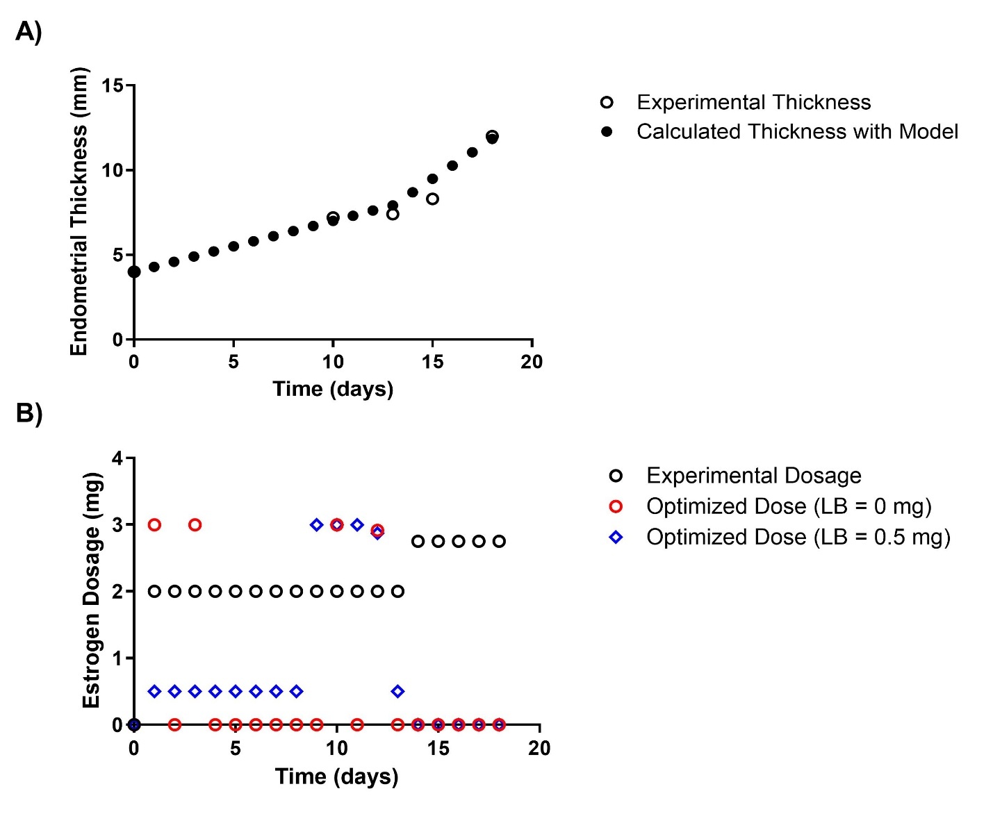
An example patient (patient 40) was selected, and their calculated profiles and dosage optimizations are shown in Figure 1. This first patient was given a nonconstant estrogen dosage (2 mg/day for days 1-13 and 2.75 mg/day for days 14-18) in the clinical setting.

The total experimental dosage for patient 40 to achieve a final endometrial thickness of 8.3 mm was 31.5 mg. The optimized dosage, determined by the model and a lower bound of 0 mg per day, was 11.9158 mg, resulting in a 62.17% reduction in estrogen. The optimized dosage, determined by the model and a lower bound of 0.5 mg per day, was 16.3720 mg, resulting in a 48.03% reduction in estrogen.

Figure 1.Patient-specific treatment and model fit for patient 40.

(A) Comparison of experimentally measured endometrial thickness and model-predicted thickness across time (R² = 0.947). (B) Experimental estrogen dosing and optimized dosing trajectories under lower-bound constraints of 0 mg/day and 0.5 mg/day.

The \(\alpha\) values and percent reductions for all patients were calculated (Table I). The average \(\alpha\) value was 3.14 ± 0.80. The average estrogen reduction at optimized dosages was 58.95 ± 20.39% with a lower bound of 0 mg/day and 36.64 ± 14.82% with a lower bound of 0.5 mg/day. Additionally, the average difference between the estrogen reductions at the lower bound of 0 mg/day and 0.5 mg/day was 22.31 ± 10.78%.

3.2. Complied Results

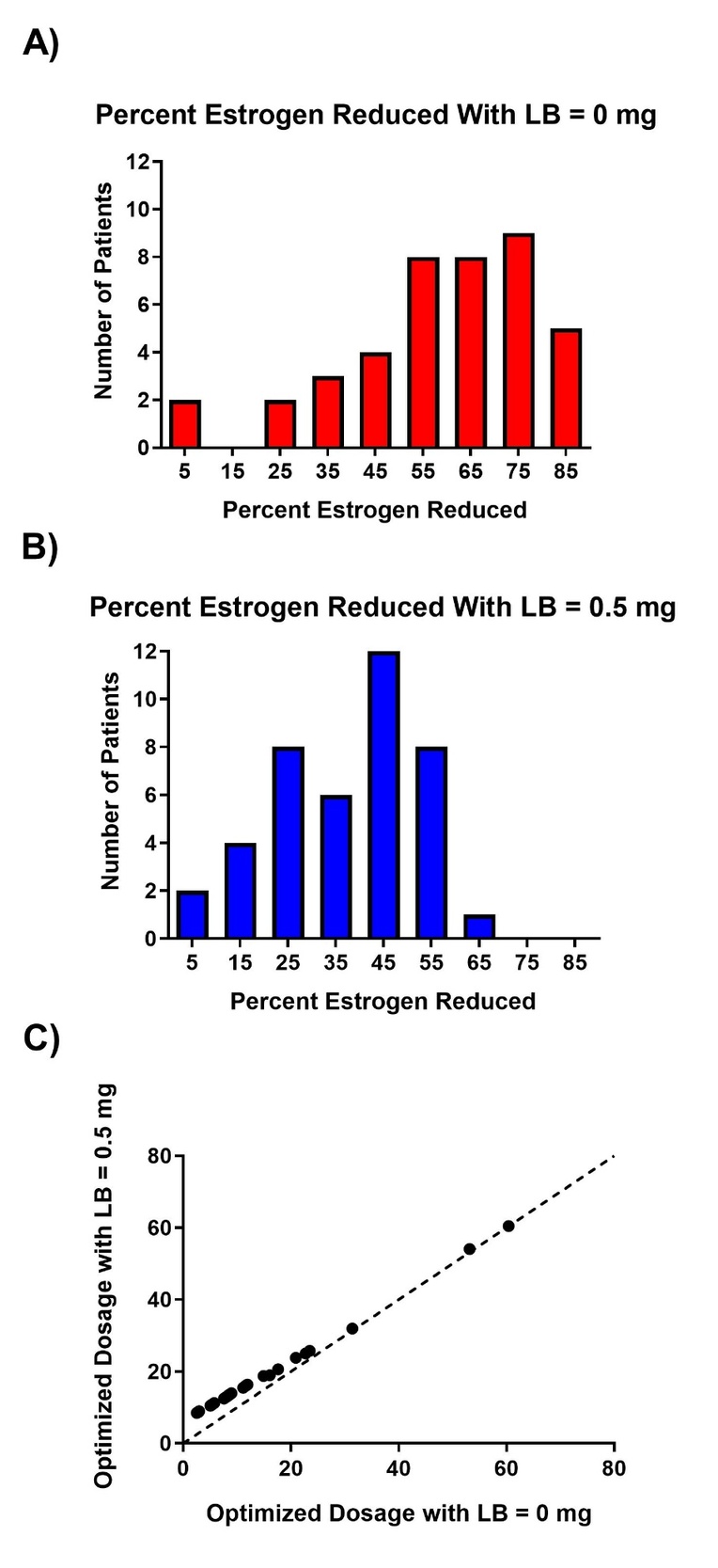
The histograms for estrogen reduction are presented in Figure 2. Compiled results are restricted to the 41 patients who were optimized to reach a final endometrial thickness of at least 8 mm. In the optimization with a lower bound of 0 mg/day (Fig. 2 A), 95% (37/39) of patients achieved an estrogen reduction of more than 30%. Two patients (marked with *) were not included in the histogram as they never reached an endometrium thickness of 8 mm in the clinical setting (final thicknesses of 7.4 mm and 7.9 mm). These patients underwent optimizations to achieve the same final thicknesses as seen in the clinical setting, resulting in reductions of 2.56% and 8.35%, respectively.

In the optimization with a lower bound of 0.5 mg/day (Fig. 2 B), 69% (27/39) of patients achieved more than 30% estrogen reduction. The two patients with final endometrial thicknesses less than 8 mm underwent optimization to achieve the same final thickness as observed in the clinical setting, resulting in reductions of 2.37% and 6.67%, respectively.

Figure 2.Distribution of percent estrogen reduction achieved under two optimization constraints: a lower bound (LB) of 0 mg/day (A) and 0.5 mg/day (B).

Histograms display the number of patients within discrete percent-reduction intervals using 10%-wide bins (e.g., 0–10%, 11–20%, etc.). Values shown on the x-axis correspond to the centers of each bin rather than the bin boundaries. Panel C shows optimized daily dosage for each individual patient under both constraints (LB = 0 mg/day vs. LB = 0.5 mg/day). The dashed 45° reference line indicates identical optimized dosages under the two conditions.

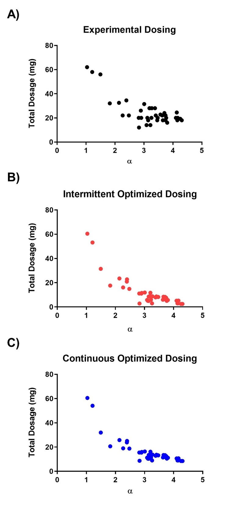
Additionally, a comparison of each patient’s \(\alpha\) value with the actual cumulative dosage and the cumulative dosage under the two optimizations is shown in Figure 3.

Figure 3.Relationship between the patient-dependent parameter α and total cumulative dosage under three dosing strategies: experimental dosing (A), intermittent optimized dosing (B), and continuous optimized dosing (C; lower bound of 0.5 mg/day).

Each point represents an individual patient, with total dosage shown in milligrams.

4. Discussion

4.1. Success of Optimization

In this study, experimental data from 47 patients was used to estimate a patient-independent growth constant (\(k\)) and patient-dependent responsiveness parameters (\(\alpha\)). The estimated \(k\) value was approximately 0.0374, while \(\alpha\) values ranged from 1.0 to 4.3, with a mean of 3.14 ± 0.80. The relatively small value of \(k\) compared to the much larger and more variable \(\alpha\) values suggests that the rate of endometrial growth is primarily governed by patient-specific responsiveness rather than a universal growth rate. This finding likely explains the substantial inter-patient variability observed in endometrial thickness vs. time profiles.

Optimized estrogen dosing profiles were also generated under two lower-bound constraints (0 mg/day and 0.5 mg/day) to compare intermittent and continuous dosing strategies. As shown in Figure 2, these constraints produced different optimization outcomes for the same patient. While some patients exhibited similar percentage reductions across both constraints, others showed markedly different reductions. Notably, every patient achieved a greater reduction in total estrogen dosage when the lower bound was 0 mg/day compared to 0.5 mg/day, with an average difference of 22.31 ± 10.78%. This systematic difference likely explains the deviation from the 45-degree reference line in Figure 2, which represents equal percentage reductions under both constraints.

A relationship between \(\alpha\) and estrogen dosage—actual clinical dosing, optimized intermittent dosing, and optimized continuous dosing—was also observed. In all three cases, an exponential relationship was identified, with R² values of 0.6815, 0.9198, and 0.8519, respectively. The optimized dosing regimens (Fig. 3, B and C) demonstrated stronger correlations with \(\alpha\) than the actual prescribed doses (Fig. 3, A), suggesting that the model imposes a tighter, more systematic relationship between cumulative estrogen dose and endometrial responsiveness than current clinical practice. Whether \(\alpha\) is associated with patient demographics or other physiological factors remains an important topic for future investigation.

The patient-specific parameter \(\alpha\) represents an individual’s endometrial responsiveness to estrogen stimulation. The wide range of \(\alpha\) values observed (1.0–4.3) highlights substantial inter-patient variability in estrogen sensitivity. Patients with higher \(\alpha\) values required less total estrogen to reach the target endometrial thickness, indicating more efficient tissue response. In contrast, patients with lower \(\alpha\) values (< 1.5) demonstrated limited benefit from optimization, suggesting that these patients may already be near their optimal dosing or may have underlying biological constraints limiting endometrial response.

Future research should investigate whether \(\alpha\) correlates with patient age and ovarian reserve, baseline hormone levels (FSH, AMH, E₂), endometrial quality or receptivity markers, previous IVF cycle outcomes, and body mass index or metabolic factors. Identifying such relationships could allow \(\alpha\) to be predicted prior to the IVF cycle, enabling prospective dose optimization rather than retrospective adjustment.

4.2. Intermittent vs. Continuous Dosing Regimens

The results indicate that intermittent dosing (lower bound of 0 mg/day) achieves significantly greater estrogen reduction, with an average decrease of 22.31% compared to continuous dosing (lower bound of 0.5 mg/day). However, several clinical considerations must be addressed before intermittent protocols can be safely implemented.

Endometrial Stability: Current clinical practice typically maintains continuous estrogen exposure to prevent endometrial regression. The safety and efficacy of intermittent dosing, including days with no estrogen administration, require prospective validation. Potential concerns include:

• Risk of endometrial shedding or breakthrough bleeding

• Loss of previously achieved endometrial thickness

• Effects on endometrial receptivity markers beyond thickness

Pharmacokinetic Considerations: Estradiol has an estimated half-life of 12–24 hours, depending on formulation. Complete cessation of dosing may result in declining serum estradiol levels and potential withdrawal effects. The current model treats estrogen administration as discrete daily inputs and does not account for pharmacokinetic carryover or steady-state behavior. Future model refinements should incorporate:

• Estradiol pharmacokinetic parameters

• Time-dependent drug accumulation

• Patient-specific clearance rates

Clinical Implementation: If future prospective studies confirm the safety of intermittent dosing, the observed average reduction of approximately 22% in estrogen usage could translate into:

• Reduced medication costs (~$12,400 per cycle based on typical pricing)¹²

• Lower incidence of estrogen-related side effects (e.g., nausea, bloating, mood changes)

• Reduced cardiovascular and thromboembolic risk in high-risk patients

Practical Recommendations: Until prospective safety and efficacy data are available, continuous dosing optimization with a 0.5 mg/day minimum may represent a more clinically acceptable strategy, while still achieving meaningful estrogen reductions (average 36.64 ± 14.82% in this cohort).

4.3. Model Validation Considerations

The mathematical model (Equation 1) assumes endometrial growth follows \(k ⋅ E^\alpha\) kinetics. While this form successfully fit 87% (41/47) of patients with adequate R² values, several limitations warrant discussion:

Model Structure: The power-law relationship was selected based on a previous study modeling follicle growth rate as a function of FSH dosage.² Alternative models considered included:

• Linear: \(\frac{dx}{dt} = k_{1}*E\) (too simplistic and does not account for individual differences in growth pattern)

• Michaelis-Menten: \(\frac{dx}{dt} = V_{\max}*E\ /(k_{m} + E)\) (assumes saturation)

• Exponential: \(\frac{dx}{dt} = \ k_{2}*e^{(k_{3}*E)}\) (poor fit in low-dose range)

The current model provided superior fit across the dosage ranges observed (2-6 mg/day).

Parameter Identifiability: With limited data points per patient (typically 3-5 measurements), estimating both \(\alpha\) and \(k\) simultaneously from individual patient data was not feasible. The population-level \(k\) estimation followed by individual \(\alpha\) estimation provided better parameter identifiability and more stable optimization.

Missing Patients (6/47): Model failure in 12.8% of patients occurred due to:

• Insufficient data points (n=4 patients had \(\leq\) 3 measurements)

• Non-monotonic growth patterns suggesting measurement error (n=5)

These patients should be analyzed separately to identify model boundaries.

Cross-Validation: Future work should include cross-validation on independent patient cohorts to assess model generalization.

4.4. Comparison to Current Clinical Practice

Current HRT protocols typically use either:

1. Fixed dosing: 6 mg/day continuously (study mean: 1.9 mg/day)

2. Incremental dosing: 2→4→6 mg/day over 12 days (study dosing: 2→2.5 mg/day or 2→6 mg/day)

Our optimized continuous protocol (0.5 mg minimum) achieved similar results with an average 36.64 ± 14.82% reduction in total estrogen dose. This suggests substantial room for dosing efficiency improvement in current clinical practice.

The variability in \(\alpha\) values (1.0-4.3) also demonstrates why fixed protocols are suboptimal. A patient with \(\alpha\)=4.3 requires only 8.5 mg total (under optimization with a lower bound of 0.5 mg/day), while protocols give them 72 mg—an approximately 8-fold excess. Conversely, patients with \(\alpha\)=1.0 may require higher doses than standard protocols provide.

This reinforces the need for personalized dosing rather than population-average protocols.

4.5. Limitations: Pregnancy Outcomes Not Assessed

A critical limitation of this retrospective analysis is the lack of correlation between optimized dosing and actual IVF outcomes (pregnancy rates, live birth rates). Achieving 8 mm endometrial thickness is necessary but not sufficient for successful implantation.

Important Caveats:

• Endometrial thickness is a surrogate marker, not a clinical endpoint

• Endometrial quality (triple-line pattern, echogenicity, vascularity) may be more predictive than thickness alone

• Over-reduction of estrogen could potentially compromise endometrial receptivity despite adequate thickness

• The optimal thickness target may vary by patient (some may need >8 mm)

4.6. Progesterone Effect

Patients were given a progesterone supplement at the end of the cycle, causing a slight decrease in endometrial thickness. Per the physician’s recommendation, this decrease was assumed to be no more than 1 mm. Since the exact value of the decrease due to the progesterone is unknown, this may lead to slight over- or underestimation of \(\alpha\) and optimized doses, particularly in patients whose final measurements occur after progesterone initiation.

4.7. Personalized Medicine Approach

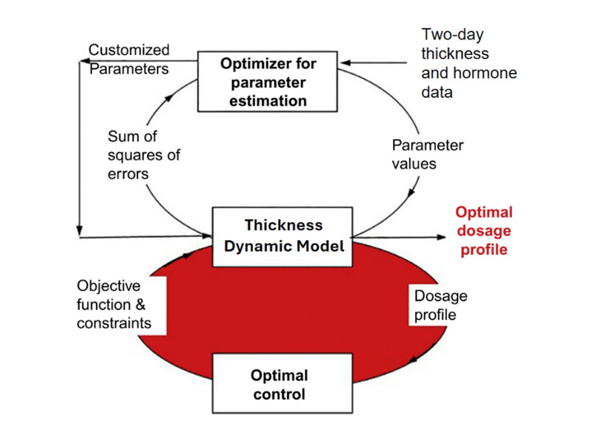
We present here a two-loop approach to personalizing and optimizing the dosage profile for future patients (Fig. 4). This is a hypothetical framework that still requires prospective validation but may be implemented in future clinical settings.

In the first loop, a patient profile is created by using thickness and hormone data (initial thickness, dosages for the first two days, experimental thicknesses for the first two days) and the patient’s independent \(k\) value to solve each patient’s \(\alpha\) value. This is done by minimizing the objective function seen below.

\[\small Sum\ of\ Squared\ Error = \sum_{i = 0}^{2}{(x_{calculated} - \ x_{experimental})}^{2}\tag{6}\]

After personalizing the model, the second loop is used to find the optimized estrogen dosage profile by solving the discretized optimal control problem.

\[\underset{C_{est}(i),\ i = 1,2,\ldots t}{Min}{\sum_{i = 0}^{T}{C_{est}(i)}}\tag{7} \]

Subject to:

\[x(t) \geq 8\tag{8}\]

\[\frac{dx}{dt} = k\ C_{est}{(t)}^{\alpha}\tag{10}\]

The constraints of this optimization model are:

• Lower bound of dosage/day = 0 mg or 0.5 mg

• Upper bound of dosage/day = 3 mg

• Maximum cycle time (T) = 13 days

• Final endometrium thickness is greater than or equal to 8 mm.

Figure 4.A two-loop optimization model for personalized dosage profiles.

Two days of initial estrogen dosage and endometrial thickness data are used to solve for customized parameters. These parameters are incorporated into the thickness dynamic model to determine an optimal dosage profile utilizing the objective function and specified constraints.

5. Conclusions

Overall, the results show that the model reduces estrogen dosing across multiple patients with varying initial conditions. Intermittent dosing appears to produce a greater percentage of estrogen reduction than continuous dosing, with an average 22.31 ± 10.78% greater reduction.

We hope to apply these findings to patients who have not yet undergone a full IVF cycle by using their initial thickness and first two-day data to predict endometrial growth and optimize estrogen dosing. Future research may also consider patient differences in the structure of each patient’s endometrial tissue. The use of AI to grade endometrial quality based on relative ratios of endometrial layers has recently shown promising results.¹³ Additionally, future research could link the \(\alpha\) value to patient parameters such as endometrial quality, initial hormonal levels, patient age, etc. This analysis, in conjunction with hormonal optimization, may lead to even better IVF outcomes.

Funding

This work was supported in part by the U.S. National Science Foundation supplement to Grant 2335090.

Conflict of interest statement

Dr. Diwekar is the owner and founder of Opt-IVF LLC.

Attenuation statements

Data related to any of the subjects in the study has not been published previously.

All study and manuscript data will be made available to the journal editors upon request before and/or after manuscript publication for review or query.

The authors followed the appropriate checklist for this study design.

CRediT authorship contribution statement

Sarah A. Lanza – Conceptualization, Data curation, Formal Analysis, Investigation, Methodology, Visualization, Writing – original draft

Urmila Diwekar – Conceptualization, Funding Acquisition, Investigation, Methodology, Validation, Writing – review and editing

Nayana Patel – Data curation, Writing – review and editing

Data Sharing Statement

Data sharing is restricted due to patient privacy protections. De-identified data is available upon request with appropriate institutional ethics approval.

Capsule

A mathematical model was developed to optimize estrogen dosing in IVF. Model predictions indicate that the total estrogen required to achieve optimal endometrial thickness is reduced, with the greatest reductions observed under an intermittent dosing regimen.